Introduction
In computer science, a Fibonacci heap is a heap data structure consisting of a collection of trees. It has a better amortized running time than a binomial heap. Fibonacci heaps were developed byMichael L. Fredman and Robert E. Tarjan in 1984 and first published in a scientific journal in 1987. The name of Fibonacci heap comes from Fibonacci numbers which are used in the running time analysis.
A Fibonacci heap H is a collection of heap-ordered trees
that have the following properties:
1. The roots of these trees are kept in a doubly-linked list (the root list of
H),
2. The root of each tree contains the minimum element in that tree (this
follows from being a heap-ordered tree),
3. We access the heap by a pointer to the tree root with the overall min-
imum key,
4. For each node x, we keep track of the degree (also known as the order
or rank) of x, which is just the number of children x has; we also keep
track of the mark of x, which is a Boolean value whose role will be explained later.

Fig. : A detailed view of a Fibonacci Heap. Null pointers are omitted for
clarity.
For each node, we have at most four pointers that respectively point to the
node’s parent, to one of its children, and to two of its siblings. The sibling
pointers are arranged in a doubly-linked list (the child list of the parent
node). We have not described how the operations on Fibonacci heaps are
implemented, and their implementation will add some additional properties
to H. The following are some elementary operations used in maintaining
Fibonacci heaps:
Inserting a node x: We create a new tree containing only x and insert it
into the root list of H; this is clearly an O(1) operation.
Linking two trees x and y: Let x and y be the roots of the two trees we
want to link; then if key(x) ≥ key(y), we make x the child of y; otherwise,
we make y the child of x. We update the appropriate node’s degrees and the
appropriate child list; this takes O(1) operations.
Cutting a node x: If x is a root in H, we are done. If x is not a root in
H, we remove x from the child list of its parent, and insert it into the root
list of H, updating the appropriate variables (the degree of the parent of x
is decremented, etc.). Again, this takes O(1) operations. We assume that
when we want to cut/find a node, we have a pointer hanging around that
accesses it directly, so actually finding the node takes O(1) time.

Fig.1: The Cleanup algorithm executed after performing a delete-min
Marking a node x: We say that x is marked if its mark is set to true, and
that it is unmarked if its mark is set to false. A root is always unmarked.
We mark x if it is not a root and it loses a child (i.e., one of its children is
cut and put into the root-list). We unmark x whenever it becomes a root.
We shall see later on that no marked node will lose a second child before it
is cut itself.
The delete-min Operation
Deleting the minimum key node is a little more complicated. First, we remove
the minimum key from the root list and splice its children into the root list.
Except for updating the parent pointers, this takes O(1) time. Then we scan
through the root list to find the new smallest key and update the parent
pointers of the new roots. This scan could take O(n) time in the worst
case. To bring down the amortized deletion time (see further on), we apply
a Cleanup algorithm, which links trees of equal degree until there is only
one root node of any particular degree.
Let us describe the Cleanup algorithm in more detail. This algorithm
maintains a global array B[1 . . . ⌊log n⌋], where B[i] is a pointer to some
previously-visited root node of degree i, or Null if there is no such previously-
visited root node. Notice, the Cleanup algorithm simultaneously resets the
parent pointers of all the new roots and updates the pointer to the minimum
key. The part of the algorithm that links possible nodes of equal degree is
given in a separate subroutine LinkDupes, see Figure 1. The subroutine ensures that no earlier root node has the same degree as the current. By the
possible swapping of the nodes v and w, we maintain the heap property. We
shall analyze the efficiency of the delete-min operation further on. The fact
that the array B needs at most ⌊log n⌋ entries is proven in Sections, where
we prove that the degree of any (root) node in an n-node Fibonacci heap is
bounded by ⌊log n⌋.
Fig.2: The Promote algorithm
The decrease-key Operation
If we also need the ability to delete an arbitrary node. The usual way to do
this is to decrease the node’s key to −∞ and then use delete-min. We start
by describing how to decrease the key of a node in a Fibonacci heap; the
algorithm will take O(log n) time in the worst case, but the amortized time
will be only O(1). Our algorithm for decreasing the key at a node v follows
two simple rules:
1. If newkey(v) < key(parent(v)), promote v up to the root list (this
moves the whole subtree rooted at v).
2. As soon as two children of any node w have been promoted, immedi-
ately promote w.
In order to enforce the second rule, we now mark certain nodes in the Fi-
bonacci heap. Specifically, a node is marked if exactly one of its children has
been promoted. If some child of a marked node is promoted, we promote
(and unmark) that node as well. Whenever we promote a marked node, we unmark it; this is the only way to unmark a node (if splicing nodes into the
root list during a delete-min is not considered a promotion). A more formal
description of the Promote algorithm is given in Figure 2. This algorithm
is executed if the new key of the node v is smaller than its parent’s key.
Amortized Analysis
In an amortized analysis, time required to perform a sequence of data struc-
ture operations is averaged over all the operations performed. Amortized
analysis can be used to show that the average cost of an operation is small,
if one averages over a sequence of operations, even though a single operation
might be expensive. Amortized analysis differs from average-case analysis
in that probability is not involved; an amortized analysis guarantees that
average performance of each operation in the worst case.
There are several techniques used to perform an amortized analysis, the
method of amortized analysis used to analyze Fibonacci heaps is the potential
method. When using this method we determine the the amortized cost of
each operation and may overcharge operations early on to compensate for
undercharges later. The potential method works as follows. We start with
an initial data structure D0 on which s operations are performed. For each
i = 1, . . . , s, we let ci be the actual cost of the i-th operation and Di be
the data structure that results after applying the i-th operation to the data
structure Di−1. A potential function _ maps each data structure Di to a
real number _(Di), which is the potential (energy) associated with the data
structure Di. The amortized cost ˆci of the i-th operation with respect to the
potential function _ is defined by:
The amortized cost of each operation is thus its actual cost plus the increase
in potential due to the operation. The total amortized costs of the s opera-
tions is

If we can prove that _Ds ≥ _D0 , then we have shown that the amortized
costs bound the real costs. Thus, we can analyze the amortized costs to
obtain a bound on the actual costs. In practice, we do not know how many
operations s might be performed. Therefore, if we require that _(Di) ≥ _D0
for all i, then we guarantee that we pay in advance. It is often convenient to
define _(D0) = 0 and then to show that _(Di) ≥ 0.
Intuitively, if the potential difference _(Di)−_(Di−1) of the i-th operation
is positive, then the amortized cost ˆci represents an overcharge to the i-th
operation, and the potential of the data structure increases. If the potential
difference is negative, then the amortized costs represents an undercharge
and the actual cost of the operation is paid by a decrease in the potential.
Comparison of theoretic bounds of variants
The following time complexities are amortized (worst-time) time complexity for entries marked by an asterisk, and regular worst case time complexities for all other entries. O(f) gives asymptotic upper bound and Θ(f) is asymptotically tight bound (see Big O notation). Function names assume a min-heap.
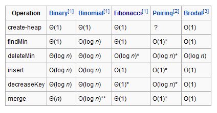
(*)Amortized time
(**)Where n is the size of the larger heap
(**)Where n is the size of the larger heap
Application
The heap data structure has many applications.
§ Heapsort: One of the best sorting methods being in-place and with no quadratic worst-case scenarios.
§ Selection algorithms: Finding the min, max, both the min and max, median, or even the k-th largest element can be done in linear time (often constant time) using heaps.[4]
§ Graph algorithms: By using heaps as internal traversal data structures, run time will be reduced by polynomial order. Examples of such problems are Prim's minimal spanning tree algorithm and Dijkstra's shortest path problem.
Full and almost full binary heaps may be represented in a very space-efficient way using an array alone. The first (or last) element will contain the root. The next two elements of the array contain its children. The next four contain the four children of the two child nodes, etc. Thus the children of the node at position n would be at positions 2n and 2n+1 in a one-based array, or 2n+1 and 2n+2 in a zero-based array. This allows moving up or down the tree by doing simple index computations. Balancing a heap is done by swapping elements which are out of order. As we can build a heap from an array without requiring extra memory (for the nodes, for example), heapsort can be used to sort an array in-place.
One more advantage of heaps over trees in some applications is that construction of heaps can be done in linear time using Tarjan's algorithm.
Heapsort
Heapsort is a comparison-based sorting algorithm to create a sorted array (or list), and is part of the selection sort family. Although somewhat slower in practice on most machines than a well implemented quicksort, it has the advantage of a more favourable worst-case O(n log n) runtime. Heapsort is an in-place algorithm, but is not a stable sort.
Heapsort begins by building a heap out of the data set, and then removing the largest item and placing it at the end of the partially sorted array. After removing the largest item, it reconstructs the heap, removes the largest remaining item, and places it in the next open position from the end of the partially sorted array. This is repeated until there are no items left in the heap and the sorted array is full. Elementary implementations require two arrays - one to hold the heap and the other to hold the sorted elements.
Heapsort inserts the input list elements into a binary heap data structure. The largest value (in a max-heap) or the smallest value (in a min-heap) are extracted until none remain, the values having been extracted in sorted order. The heap's invariant is preserved after each extraction, so the only cost is that of extraction.
During extraction, the only space required is that needed to store the heap. To achieve constant space overhead, the heap is stored in the part of the input array not yet sorted. (The storage of heaps as arrays is diagrammed at Binary heap#Heap implementation.)
Heapsort uses two heap operations: insertion and root deletion. Each extraction places an element in the last empty location of the array. The remaining prefix of the array stores the unsorted elements.
Example of Heapify
Suppose we have a complete binary tree somewhere whose subtrees are heaps. In the following complete binary tree, the subtrees of 6 are heaps:

The Heapify procedure alters the heap so that the tree rooted at 6's position is a heap. Here's how it works. First, we look at the root of our tree and its two children.

We then determine which of the three nodes is the greatest. If it is the root, we are done, because we have a heap. If not, we exchange the appropriate child with the root, and continue recursively down the tree. In this case, we exchange 6 and 8, and continue.

Now, 7 is greater than 6, so we exchange them.

We are at the bottom of the tree, and can't continue, so we terminate.
Selection algorithms
In computer science, a selection algorithm is an algorithm for finding the kth smallest number in a list (such a number is called the kth order statistic). This includes the cases of finding theminimum, maximum, and median elements. There are O(n), worst-case linear time, selection algorithms. Selection is a subproblem of more complex problems like the nearest neighbor problem andshortest path problems.
The term "selection" is used in other contexts in computer science, including the stage of a genetic algorithm in which genomes are chosen from a population for later breeding; see Selection (genetic algorithm). This article addresses only the problem of determining order statistics.
Selection can be reduced to sorting by sorting the list and then extracting the desired element. This method is efficient when many selections need to be made from a list, in which case only one initial, expensive sort is needed, followed by many cheap extraction operations. In general, this method requires O(n log n) time, where n is the length of the list.
Algorithm


Graph algorithm
An undirected graph G is a pair (V; E), where V is a [1]nite set of
points called vertices and E is a [1]nite set of edges.
An edge e 2 E is an unordered pair (u; v), where u; v 2 V .
In a directed graph, the edge e is an ordered pair (u; v). An edge (u; v) is incident from vertex u and is incident to vertex v.
A path from a vertex v to a vertex u is a sequencehv0; v1; v2; : : : ; vki of vertices where v0 = v, vk = u, and (vi; vi+1) 2E for i = 0; 1; : : : ; k 1.
The length of a path is defined as the number of edges in the path.

An undirected graph is connected if every pair of vertices is connected by a path.
A forest is an acyclic graph, and a tree is a connected acyclic graph.
A graph that has weights associated with each edge is called a weighted graph.
Graphs can be represented by their adjacency matrix or an edge (or vertex) list.
Adjacency matrices have a value ai;j = 1 if nodes i and j share an edge; 0 otherwise. In case of a weighted graph, ai;j = wi;j, the weight of the edge.
The adjacency list representation of a graph G = (V; E) consists of an array Adj[1::jV j] of lists. Each list Adj[v] is a list of all vertices adjacent to v.
For a graph with n nodes, adjacency matrices take T heta(n2) space and adjacency list takes (jEj) space.

Worst case
Although the total running time of a sequence of operations starting with an empty structure is bounded by the bounds given above, some (very few) operations in the sequence can take very long to complete (in particular delete and delete minimum have linear running time in the worst case). For this reason Fibonacci heaps and other amortized data structures may not be appropriate for real-time systems.
Conclusion
We were ultimately able to get this asymptotic improvement because insert, findMin, and decreaseKey using FHeaps are only O(1) amortized. 3 Unfortunately, FHeaps aren't often used in practice due to the difficulty of implementing them efficiently. They are also avoided in real time systems because there can be some operations that take substantially longer than others, which may not be acceptable in the environment. For these reasons, FHeaps have been mostly of theoretical interest and have inspired many other fast priority queue supporting data structures. One such example are Brodal Queues which are also quite complicated; however, they provide the same time bounds as FHeaps only unamortized! This makes them an attractive candidate for real time systems.
Reference
- Thomas H. Cormen, Charles E. Leiserson, Ronald L. Rivest, and Clifford Stein. Introduction to Algorithms, Second Edition. MIT Press and McGraw-Hill, 2001. ISBN 0-262-03293-7. Chapter 20: Fibonacci Heaps, pp.476–497. Third edition p518.
- Iacono, John (2000), "Improved upper bounds for pairing heaps", Proc. 7th Scandinavian Workshop on Algorithm Theory, Lecture Notes in Computer Science,1851, Springer-Verlag, pp. 63–77
- Thomas H. Cormen, Charles E. Leiserson, Ronald L. Rivest (1990): Introduction to algorithms. MIT Press / McGraw-Hill.